| UI | MATHSim | MATHFlow | MS Visio | MATHView | ||||
|---|---|---|---|---|---|---|---|---|
| Execution | Simulation Engine | MATHFlow Repo Mgmt | MATHFlow macros | Gephi | ||||
| MATH<-> BPMN Translator | ||||||||
| Storage | BPMN Files | MATH Database | ||||||
| Microsoft Access | ||||||||
MATHSim requires .NET 4, as well as a working installation of MATHFlow 3.
MATHSim has been primarily tested on Windows 7, but Windows XP or Windows Vista should work just as well.
First, verify that MATHFlow 3 is already installed on your computer. The MATHSim installer will update MATHFlow's simulation libraries when it installs, so it is important that MATHFlow be installed first.
If you have a version of MATHSim previous to 0.3.281.0 installed, you will need to uninstall it using the Programs and Features Windows Control Panel before installing a newer version.
Then, retrieve the setup file from http://parvac.washington.edu/nccd/download/installers/MathVS-Setup.msi, and run it.
To start MATHSim, select its icon from the All Programs menu.
MATHSim can also be started from within MATHFlow; see the MATHFlow manual. In that case, MATHSim will not include a File menu, since all file operations are controlled by MATHFlow.
MATHSim can load models from two different sources: from a MATH repository, or from a BPMN-2 XML file.
BPMN is a standard for business process modeling developed and maintained by the OMG; MATHFlow generates models in a subset of BPMN that has been extended to include different information resource types and simulation information. Both the BPMN standard and a number of examples are available online. To find out more about BPMN, see the BPMN standards site.
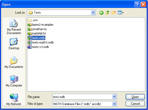
To open a model from either of these sources, select Open from the File menu, and select the file containing the model you wish to open.
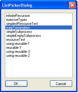
If the file you have selected is a MATH repository, you will be further prompted to choose the model from those present in the repository.
When a model is being loaded, MATHSim may display warnings concerning disconnected flows, empty resource sets, or other problems with the model. These warnings will not prevent the simulator from running the model, but they may very well prevent it from running as intended, so it is important to review these warnings before proceeding.
Whenever possible, MATHSim will correct
the model to address
the causes of the warnings. For example, disconnected flows are
removed, and empty resource sets are provided with a resource
(Participant) so that they are no longer empty.
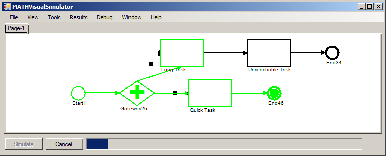
Once you have a model open, the model should appear in the model window as shown in the figure below.
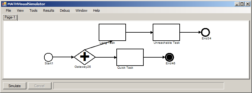
To see the different process contexts the model contains, select the different tabs along the top of the modeling window.
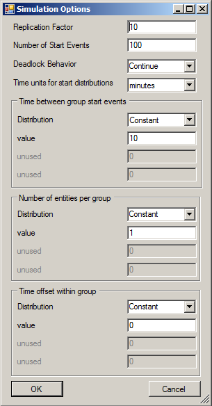
Before you run a simulation of the model, you may want to adjust the simulation parameters. For the most part, the behavior of the model under simulation is already encoded in the model itself, and to edit those parameters you will need to change the model in MATHFlow. MATHSim, however, allows you to change the number of independent trials in the simulation (replication factor); how many entities (tokens) should pass through the system to make up one trial; and how quickly new tokens are started within a trial.
For example, let's say that the process you are modeling is of patient check-in at a clinic. There are n greeters at the check-in desk, and it takes each of them m minutes to process a patient. Quantity p patients arrive every day, one every ten minutes according to the clinic's appointment book, but some are early and some are late. In our simplistic model, patients wait until they are processed, no matter how long that takes; and once they are processed, they are no longer of concern to this part of the model.
A single trial for this scenario represents a single day of checking in patients. The Replication Factor determines how many days we want to simulate, in order to determine what the average day looks like (or best, or worst, or 10th-percentile, etc.). The Number of Start Events determines how many patients are on the schedule each day; in the model above, this is given by p. Finally, the Time between start events determines the interval between patients actually arriving, within a given day; in the model described above, this might be given by a normal distribution with a mean of 10 minutes and a standard deviation of 5 minutes.
The default setting for Units is minutes, regardless of what might have been entered in the model in MATHFlow.
These simulation parameters can be set in the Simulation Options dialog in the Tools menu.
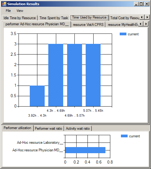
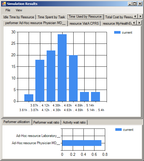
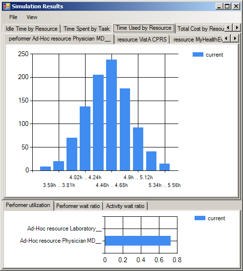
It is important to note the difference between replication factor and number of start events. The replication factor simply states how many runs the simulator should make. Because these runs are independent, a larger replication factor will not change the results, though it should make them more accurate. Three different runs with different values of replication factor are shown below. As the number of samples increases from 10 to 100 to 1000, a smooth distribution emerges, though the modal value remains close to 4.5 hours.
Number of start events, however, will change the results, since it changes the number of tokens in the system during any given trial. Doubling the number of start events, for example, could be expected to double the total cost and the total time.
Deadlock Behavior allows you to change what happens when a deadlock occurs in the simulation. By default, this value is set to Continue, meaning that the results from the current trial are discarded and a new trial is begun. If you are trying to debug a deadlock situation, however, it may be more useful to set this value to Stop, which will instead halt all simulation as soon as the first deadlock is detected. The simulation log will be shorter and easier to comprehend in the second case.
The Time between group start events control sets the time between group start events (usually, between token start events). This is fairly straightforward, but the distribution list does have one subtlety that is worth mentioning. In general, the distribution that is chosen will specify the time between start events. If N-at-a-time is chosen, however, the behavior will be somewhat different. This so-called distribution will instead release a new token into the model whenever the number of live instances falls below N, assuming that the total number of instances has not already been reached. If N=1, this means that only one instance will be active in the model at any given time. Because the run queue is limited to N elements, running with N-at-a-time with N=1 is the fastest way to run a model, assuming of course that one entity at a time is a valid scenario for the model in question.
Note that, although you can also change the nominal timing of start events using the start object's properties, as described below, those changes will not affect the simulation unless the model is saved and reloaded. Therefore, it is a better idea to control the start timing for the model using the Simulation Options dialog.
Number of Entities per Group and Time offset within
group allow the modeling of bursty
start distributions.
If the number of entities per group is greater than one, a single
token will be started at the given time. If it is set greater than
one, however, the number of tokens specified will be started at every
larger-scale start event; these tokens will have their start time
offset by the Time offset within group distribution.
For example, to start four tokens at a time, normally distributed within that group of four with a standard distribution of five minutes, but each group of four should be centered on the hour, you would set Time between group start events to Constant: 60 minutes; Number of entities per group to 4; and Time offset within group to Normal, SD 5 minutes.
Once you have set the simulation parameters the way you want them, click on the Simulate button to start the simulation.
While the simulation is running, you should receive three different types of feedback:
token, traverses the model, pausing where the model delays it or where resource contention causes a delay. The time for this token is non-linear, that is, the tokens should move in the right order, but an hour delay is the same for them as a momentary delay. These tokens serve to give you a basic idea of how control passes through your model, as well as where resource contention exists within the model.
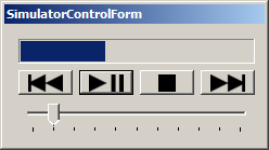
You will also see a VCR controls
control panel, which allows
you to pause, restart, and change the speed of the animation
displaying the tokens. It is important to realize that the simulation
is in fact running much more quickly than the animation is displayed;
so speeding up the animation will not make the simulation proceed any
more quickly, and pausing it will not make the simulation complete any
more slowly.
Pressing Stop on the VCR controls, however, will cancel the simulation.
When tokens are within an activity, they are displayed as attached
to the left-hand side of the activity; for example, in the figure,
there is a token engaged in the Quick Task
activity. If more than
one token is engaged in the activity at the same time, the size of the
disc is scaled according to the logarithm of the number of tokens
present.
When tokens are waiting for resources required to perform an activity, however, they are displayed in a queue extending to the left of the activity, about a quarter of the way from the top.
When tokens move from one activity to another, they follow a straight line between the center of the left-hand-side of the first activity to the center of the left-hand side of the second; regardless of where the flow arrow may be displayed.
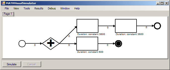
Once a model is loaded, it may be useful to see an overview of what each activity costs and how long it takes, as well as what the probabilities are on each of the flows. These and other overlays are contained in the View menu. In the example shown below, the task names have been turned off, and probabilities and durations turned on. A quick visual scan tells us that all flows have equal probability (0/0 = 1, for this purpose) and the task labeled quick task
above can be seen to be, in fact, of shorter duration than the others.
To see a summary of the information attributes used by each task, both input and output, select Information Resource Use by Activity from the Window menu. The summary provides a straightforward summary of which information attributes are needed by, and provided by, each task, as well as what information resources store those attributes, and what values, if any, are assigned.
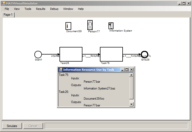
In the figure, the first task ("Task26") reads the value of foo from Document39 when it begins, and writes attribute bar to human information resource Person77 when it completes. Likewise the second task ("Task75") reads attribute bar back from the human information resource Person77 and writes attribute baz to Information System27 when it completes.
MATHSim includes limited capabilities for editing a model, including the creation of a model from scratch. These capabilities may prove useful should a model generated in MATHFlow prove to be corrupted.
In the Window menu, select the Tool Palette item. This brings up the tool palette containing the stencils.
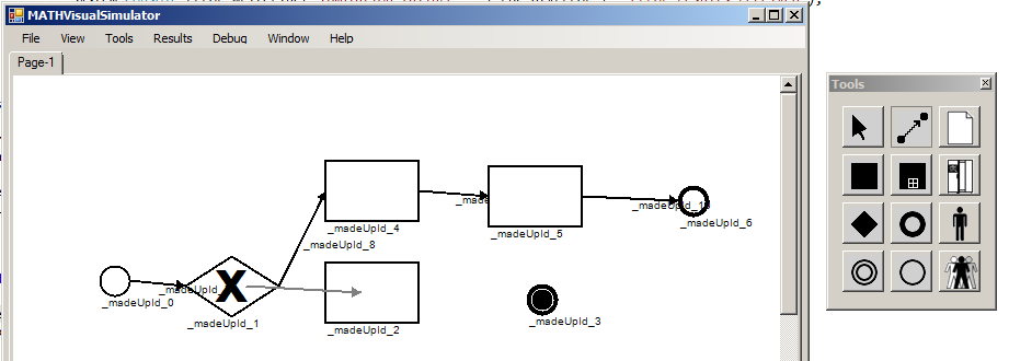
The default tool is the pointer tool, which allows you to grab any non-flow object and move it around on the page. Also, a double-click with this tool will allow you to navigate down into subprocesses.
The other tools allow you to create various types of objects on the page by clicking.
An exception is the Flow tool; this allows you to join two already existing objects with a flow. To use this tool, first select it from the tool palette. Then click on any object, and drag toward another object. You will see a grey arrow trailing behind your mouse. Drag the head of this arrow onto another object, and release the mouse button. The grey arrow should be replaced by an ordinary black flow object.
Regardless of which tool you have selected, right-clicking on an object will allow you to edit the properties of that object, or to delete the object. If the object is an intermediate event node, you can also attach it to a task or subprocess as a boundary event.

Process objects cannot be renamed through their properties; to rename a Process object, you must use the Rename Process option on the context menu.
Right-clicking on an Event object will also allow you to attach that Event to a Process or Task object as a boundary event, or to detach an Event from a Process or Task. Boundary timers can limit the run time of a subprocess, and other types of boundary events can define alternative exit paths from a process, depending on the exit conditions; see page 277 of the BPMN 2.0 specification for details.
Finally, you can navigate back to the containing process context by right-clicking on the background, and selecting Navigate Up One Level. (You can always navigate to a different process context using the tabs; Navigate Up One Level allows you to go specifically to the context containing the subprocess you are looking at.)
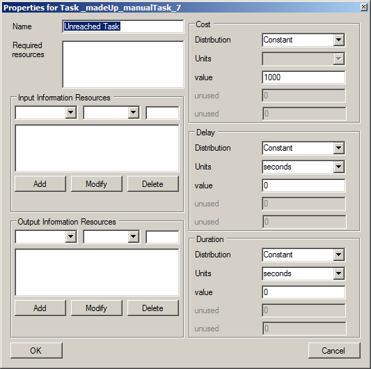
Certain classes of BPMN objects have properties specific to their class, which change the behavior of the model.
The subprocess object has three such properties: Entry Assertion, Exit Assertion and Loop While. Entry Assertion contains an expression which, if not empty, must evaluate to a non-zero value in order for a token to enter the subprocess. Exit Assertion is similar, but the expression is evaluated on exit. Both of these expressions are evaluated in terms of information variables set by tasks in the model; they allow the simulator to verify that the expectations of the model designer are accurate.
Loop While specifies an expression which, if it evaluates to a non-zero value, causes a token leaving the subprocess to instead re-enter it.
The expressions referred to above are arithmetic expressions, optionally containing variables of the form InformationResourceName.attributeName. Tasks can set the value of these attributes using the same type of expression (see Adding Information Resources in the MATHflow manual).
The arithmetic expressions are implemented using the NCalc library, so it understands all of these operators (specified from low to high precedence): || && == != < <= > >= + -[binary] * / % & | ^ << >> ! ~ -[unary] (), as well as common mathematical functions (abs, exp, pow, sign, sin, sqrt, etc.)
Event objects allow the specification of Type (Start, End or Intermediate); Subtype, of which there are many; and Throwing/Catching, which specifies whether they generate a thrown event signal or whether they consume such a signal. (Note that End Events are always Throwing, regardless of the setting of the T/C property.)
In addition, events of message subtype have an additional property, Class, which allows the association of event objects together. When a message is thrown from an event object of class A, only event objects of class A attached to super-processes of the process containing the thrown event will catch that thrown event.
Finally, event objects of subtype link allow the specification of the other side of the link.
MATHSim has several save as
options, all located in the File menu:
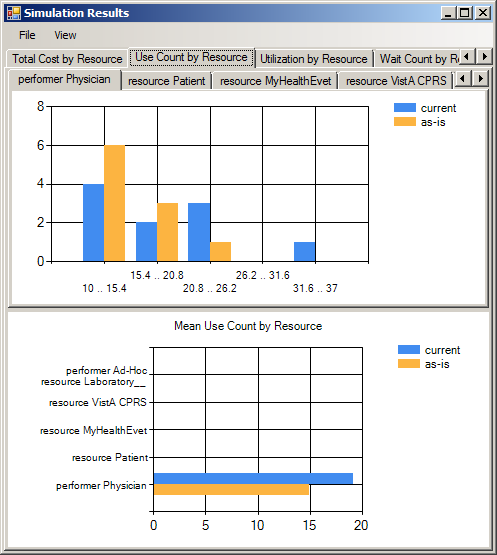
When the simulation completes, a viewer window will open displaying histograms of each of the measures recorded during the simulation.
The different types of measures recorded are:
When one of these categories is selected on the top row of tabs, a second row of tabs will appear, showing a histogram of the measure in question applied to the given task (or resource). For example, in the figure below, the user has selected Use Count by Resource, and the resource (performer) Physician, displaying a histogram of the number of times the Physician resource was used during a given run.
In these histogram displays, MATHSim distinguishes between
variables that represent time, and those that are in other units
(dollars, liters, fathoms, etc.). The default display for time
variables is fractional hours; to change this to integer seconds or
to use the standard
Microsoft time interval notation, select the
appropriate formatter from the
View menu.
Below this second set of tabs is a second chart, showing the mean value for the chosen category, for all tasks (or resources). This allows you to compare between different tasks or resources easily, as well as explicitly providing the mean value, which is not easily discerned from a histogram. Time in this second display is always shown in integer seconds.
In addition to these per-task and per-resource measures, there are four global measures that are computed by the simulator: cycle time, startTime, cost, and taskCount. Cycle time shows the sum of the individual time-to-completion for each starting token; taskCount counts the number of times a token entered a task (any task, including processes); startTime records the times that tokens entered the simulation; and cost calculates the total cost. Cycle time and cost may be valuable results in and of themselves; startTime and taskCount are primarily useful for debugging a model.
To compare runs of similar models (e.g., an as is
versus
a to be
model, or perhaps the same model run with different
simulation parameters), first generate the results from the first
model, and open the results window. From the results
window's File menu, select Save Current
for
later comparison. Then run the second model, and open the
results window. Go back into the File menu, and
select Open for comparison. Select any of the results
files you have saved previously; those results will be added to the
histogram alongside the current results. The results
marked current always refer to the results of the most
recent run; the results of previous runs will be displayed will be
displayed under their filename.
It is important, of course, that the variables to be compared have the same name.
The histograms are only meant as a preview of the data available from the simulation. To save it for consumption by a data analysis package, select Save Results As... from the Results menu. The resulting file (CSV or xls) can be opened in Excel or many other applications.
Alternatively, the results can be opened directly in Excel using the Open in Excel option from the Results menu.
If you find that you need to answer more complex questions than the provided results allow for, you may be able to find the data you are looking for in the simulation log. Every action taken by every token during the course of a simulation run is recorded in the log. After running a simulation, you can see the log by selecting Simulation Log from the Results menu.
The simulation log is formatted as a text file; each line describes a single event. An example line is
3650: token 0.0.0.0.0 use amount 3610 of resource 'Resource46' at node 'Task28', with a cost of 0
This line says that at 1:00:50 after the start of simulation, the token with the designation 0.0.0.0.0
finished using the resource Resource46
after holding it for 1:00:10; that this event occurred at node Task28
, and that the cost incurred by this resource usage was 0.
Node labels in the log are presented as human-readable labels if the modeler has supplied them; otherwise the node IDs are used. Note that, while the node IDs are guaranteed to be unique within the model, the human-readable labels are not.
The token labels are constructed as follows. The first number is
the trial number, and the second is the instance number. The third
number is always zero. Thus, the first token in every simulation log
will be 0.0.0
. Whenever control enters a subprocess, the token goes
to sleep, creating a new child token in the subprocess context. The
child token has the same label as the parent, with .0
appended. If
sibling tokens are ever created, for example, at a parallel Split
gateway, the last number is incremented for each new sibling.
Note that, while token creations are not recorded, token deletions
are always explicitly recorded. Thus, while there may during the
course of a simulation be several tokens all with the same label,
these will never coexist, and a token deleted
event will always
be recorded in between.
The following transcript records a single instance of the early
termination
test model. Note the creation of a sibling token at
time 30, and the deletion of both tokens at time 3670, when token
0.0.0.0.0 enters the terminating End Event.
0: token 0.0.0 delay at node '___theMetaNode'
0: token 0.0.0 enter node '___theMetaNode'
0: token 0.0.0.0 delay at node 'Page-1'
0: token 0.0.0.0 enter node 'Page-1'
0: token 0.0.0.0.0 delay at node 'Start1'
0: token 0.0.0.0.0 enter node 'Start1'
10: token 0.0.0.0.0 exit node 'Start1'
10: token 0.0.0.0.0 delay at node 'terminateTest___Page-1___Flow'
10: token 0.0.0.0.0 enter node 'terminateTest___Page-1___Flow'
20: token 0.0.0.0.0 exit node 'terminateTest___Page-1___Flow'
20: token 0.0.0.0.0 delay at node 'Gateway26'
20: token 0.0.0.0.0 enter node 'Gateway26'
30: token 0.0.0.0.0 exit node 'Gateway26'
30: token 0.0.0.0.1 delay at node 'terminateTest___Page-1___Flow.31'
30: token 0.0.0.0.1 enter node 'terminateTest___Page-1___Flow.31'
40: token 0.0.0.0.1 exit node 'terminateTest___Page-1___Flow.31'
30: token 0.0.0.0.0 delay at node 'terminateTest___Page-1___Flow.29'
30: token 0.0.0.0.0 enter node 'terminateTest___Page-1___Flow.29'
40: token 0.0.0.0.0 exit node 'terminateTest___Page-1___Flow.29'
40: token 0.0.0.0.1 delay at node 'Long Task'
40: token 0.0.0.0.1 enter node 'Long Task'
40: token 0.0.0.0.0 delay at node 'Quick Task'
40: token 0.0.0.0.0 enter node 'Quick Task'
3650: token 0.0.0.0.0 exit node 'Quick Task'
3650: token 0.0.0.0.0 delay at node 'terminateTest___Page-1___Flow.45'
3650: token 0.0.0.0.0 enter node 'terminateTest___Page-1___Flow.45'
3660: token 0.0.0.0.0 exit node 'terminateTest___Page-1___Flow.45'
3660: token 0.0.0.0.0 delay at node 'End46'
3660: token 0.0.0.0.0 enter node 'End46'
3670: token 0.0.0.0.0 deleted
3670: token 0.0.0.0.1 deleted
3670: token 0.0.0.0 exit node 'Page-1'
3680: token 0.0.0.0 deleted
3680: token 0.0.0 exit node '___theMetaNode'
3690: token 0.0.0 deleted
As tokens move through the model, the parameters of the activities through which they move affect their behavior, as do conditions elsewhere in the model. This is a summary of what happens as a token passes through an activity. Not all of these steps apply to every type of activity.
If the activity in question is a Task that has a Delay parameter,
the token will adjust its notion of current time
to account for the
delay before proceeding. If this causes this token no longer to be
the earliest active token, the actions of the other (earlier) active
token will preempt this token.
If the activity is a joining And
gateway, the gateway will
collect as many tokens as the gateway has inputs, and only then allow one
of the tokens to proceed while destroying the others.
When tokens are merged, the surviving token takes on all of the accumulated cost(s) of any tokens that were destroyed.
If the activity is a Task that is the recipient of a Message Flow, the token will wait until the Task receives a message allowing it to proceed. If a message has already been received, the token continues uninterrupted.
The token will attempt to seize all the resources required by a Task. In the event that some of the resources are unavailable, the token will release the resources it was able to acquire, if any, and wait until all the resources it needs are available before proceeding.
When MATHSim loads models from MATHFlow, all types of Information Resources are interpreted as required resources, with the exception of Information Systems. Task Performers are also considered to be required resources.
Increment the Hit Count for this Task. If we had to wait before entering, increment the Wait Count and update the Wait Time, both for the Task being entered and for the resource that had to be waited for. (It may be, if the token required more than one resource but both were unavailable for the same period of time, that only the first will be charged.)
The token records an access to the input information resources.
Any timers attached to this activity will be started.
The token's notion of current time
is updated to reflect the
task's duration. As above, if this causes the token not to be the
earliest active token, another token may preempt this one.
Any timers attached to this activity will be canceled.
The token records an access to the output information resources.
Any resources reserved for the duration of a Task are released.
The token is charged at this point for the cost of the task. In addition, the taskCount parameter is increased by one, since one task has been completed.
If the activity is a Send Task or a Throwing
Message Intermediate
Event, a message is generated and sent to the other end of the Message
Flow.
The token transitions to the outgoing flow. In the case that the
activity is a Split gateway, the behavior depends on the type of
gateway. And
gateways send the existing token along the first
flow, and create new sibling tokens to send along all the other
outbound flows. Or
gateways consult the probabilities of each
outgoing flow and send a token along the flow, or not, according to
the probabilities. Exclusive
gateways choose a single outgoing path
at random, according to the outbound flow probabilities, and send a
single token along the flow that was selected. Complex
gateways
follow the behavior described in
the Complex Gateways
section of the MATHFlow manual.
MATHSim, as well as being a standalone application, can be referenced as a library from another application (as it is referenced from MATHFlow). This API is described in the developer documentation.
Static methods for checking the consistency of a MATH model or an entire MATH repository are also included.
An example of how MATHSim might be called as a library from a C# program is as follows (see the documentation for details):
using [...]
using MATHVisualSimulatorLib;

namespace MyNamespace
{
    // Class must implement the ISaveAsProvider interface
    class myClass : ISaveAsProvider
    {
        IMathSimulatorForm m_sim = null;
        bool m_haveResults = false;
        bool m_haveModelLoaded = false;

        void myMethod()
        {
            // Create an IMathSimulatorForm object
            m_sim = MathSimulatorFactory.create();

            // Optionally add our own menu to the simulator.
            // In practice you might not add any menus at all.
            // m_sim.InsertMenu(0, someToolStripMenuItemWeCreated);

            // Register us as a SaveAsProvider
            m_sim.register(this);
        }

        /*
         * Event handlers
         */

        // Open the simulator window
        void someMenuItem_Click(object senter, EventArgs e)
        {
            m_sim.getAsForm().Show();
        }

        // When the new menu item we added is clicked, do this
        void newToolStripMenuItem_Click(object sender, EventArgs e)
        {
            m_sim.newDocument();
        }

        [... and several very similar menus for the other functions...]

        /*
         * In response to some other stimulus, myClass will call the
         * following function, to make m_sim load a MATH model from
         * a database file
         */

        // Open a MATH model in the simulator
        void openModelInSimulator(string dbFilename, string modelName)
        {
            LinkedList<string> errlist = new LinkedList<string>();
            string tmpFilename = m_sim.math2bpmn(dbFilename, modelName, null, false, errlist);
            if (tmpFilename == null)
                return;
            if (errlist.Count > 0)
                myDisplayErrlist(errlist);
            m_sim.loadBpmn(tempFilename);
            System.IO.File.Delete(tempFilename);
        }

        /*
         * ISaveAsProvider interface functions: enable and disable "Save as X"
         * menu options, in response to availability of data for those
         * operations.
         */
        public void enableSaveResults()
        {
            m_haveResults = true;
            mySaveResultsToolStripMenuItem.Enabled = true;
        }

        public void enableSaveBPMN()
        {
            m_haveModelLoaded = true;
            mySaveAsToolStripMenuItem.Enabled = true;
        }

        public void disableSaveResults()
        {
            m_haveResults = false;
            mySaveResultsToolStripMenuItem.Enabled = false;
        }

        public void disableSaveBPMN()
        {
            m_haveModelLoaded = false;
            mySaveAsToolStripMenuItem.Enabled = false;
        }
    }
}
MATHSim implements a Monte Carlo simulation, running several independent trials, each of which contains several process instances that may or may not interfere with one another's operation. The random numbers needed for Monte Carlo simulation are provided by a strong pseudo-random number generator, and the process state is maintained by a discrete event queue.
The pseudo-random numbers used in MATHSim are generated using the Mersenne Twister algorithm.
To provide random variates for most other distributions, a random number is selected on the half-open interval [0,1), which interval is mapped to the support of the particular probability distribution using the inverse cumulative function for that distribution. See a more detailed description in Banks et al., or on Wikipedia. The exception is the Poisson distribution, for which we use the acceptance-rejection method from Knuth, volume 2.
MATHSim's event scheduling is roughly based on the process scheduling algorithm of BSD Unix, though modified somewhat for efficiency in the simulation context; it can be described briefly as follows.
Each token has a notion of its current time, and its state. Time is measured in seconds since the simulation started, and state takes on various values depending on whether a token is runnable right now, is being delayed before entering a task, is waiting for resources, etc.
At the beginning of a simulation run, one token is created for
every instance
; its status is active, and
its time is set according to the specified inter-arrival
time.
The active tokens are stored in a queue, ordered by time. The implementation of this queue uses a splay tree of linked lists of tokens, in which every token in a given linked list has the same time, and the splay tree's comparison function compares the time of the linked lists.
At each step in the simulation, the scheduler removes the first (earliest) token from the active queue, performs whatever function is appropriate to its context, and then, if it remains active, replaces it in the queue. In either case, if the function that was performed had a duration, the token's time attribute is updated before its replacement in the active queue. The simulation has completed when the active queue becomes empty. If any inactive tokens remain, the run has become deadlocked, and its results are discarded.
There are four ways that a token could become inactive: it could require resources that are not currently available; it could be the parent of other tokens that operate in a subprocess context, waiting for the child tokens to terminate; it could be waiting for a message to proceed; or it could be waiting for sibling tokens to arrive at a merge gateway. If a token's action causes its state to become one of these states, it is not replaced in the active queue.
If, during its action, a token causes other, inactive, tokens to become active, they are placed in the queue with their time set to the same value as the activating token. Each context that might keep a token from being active (a resource, a merge gateway, a process, etc.) maintains its own list of tokens whose activity it is suppressing, so that these tokens can be easily located when circumstances allow them to activate.
Insertion and deletion of elements from splay trees both have average O(log n) and worst-case O(log2n) operation. Since there are n tokens total, and all of them must run somehow in order for the simulation to complete, the average operation of the simulator will be O(n log n) in the number of tokens started, with a worst case of O(n log2n).
Banks, J. and Carson, John S. II (1984) Discrete-Event System Simulation. Prentice-Hall.
Business Process Model and Notation (BPMN), Version 2.0. Technical Report, Object Management Group, January 2011.
Jones, Douglas W. (1986) Empirical Comparison of Priority Queue and Event Set Implementations. Communications of the ACM, 29, April 1986, pp. 300–311.
Knuth, Donald E. (1969). Seminumerical Algorithms. The Art of Computer Programming, Volume 2. Addison Wesley.
Matsumoto, M. and Nishimura, T. (1998). Mersenne twister: a 623-dimensionally equidistributed uniform pseudo-random number generator. ACM Transactions on Modeling and Computer Simulation 8 (1): 3–30.