| UI | MATHSim | MATHFlow | MS Visio | MATHView | ||||
|---|---|---|---|---|---|---|---|---|
| Execution | Simulation Engine | MATHFlow Repo Mgmt | MATHFlow macros | Gephi | ||||
| MATH<-> BPMN Translator | ||||||||
| Storage | BPMN Files | MATH Database | ||||||
| Microsoft Access | ||||||||
MATHView requires Java JRE6, available from http://www.java.com/en/download/.
MATHView is a collection of plugins that runs within the Gephi graph visualization platform; thus, installing MATHView also installs Gephi. To install Gephi with the MATHView plugins, download the zip archive file from http://parvac.washington.edu/nccd/download/installers/gephi.zip, and unpack it somewhere on your computer.
Once the zip file is unpacked, you can run Gephi/MATHView using the gephi.exe file in the bin folder.
When Gephi runs the first time, it may complain about a list of plugins it wants to disable. Of the two options presented, you should choose "Disable and continue".
The rest of this section is optional, but may prove useful if you should later wish to extend or configure Gephi.
Gephi can be extended by loading in plugins, extra modules that have been designed to work in this environment. Gephi has a built-in plugin manager that derives from the plugin capabilities built into the Netbeans application platform. This manager will automatically attempt to connect to the plugin catalogs hosted at the main Gephi site.
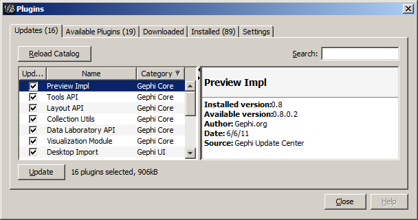
To use the plugin manager, select Plugins from the Tools menu. This will display a window that contains five tabs: Updates, Available Plugins, Downloaded, Installed, and Settings. Unless you are hosting your own Plugin center, you can ignore the Settings tab, as that just lists the available sites to get plugins from; it has already been set with the Gephi plugin sites. The Installed tab lists the plugins you have already installed; this will be empty at first.
The Available Plugins tab lists the plugins that could be installed. Clicking on the name of the plugin displays some information about it in the panel to the right of the plugin list—even more information about the plugin can be found at http://www.gephi.org/plugins/. Checking the box to the left of the plugin name selects it for installation. After the desired plugins have been selected, clicking the Install button will download and install them. Some plugins may require the application to restart in order to take effect, but you will now have the option of restarting immediately or deferring the restart until later.
Updates to installed plugins will be listed in the Updates tab. The Downloaded tab will have a list of plugins that have been downloaded manually and saved in your file system. These plugin files all have a .nbm extension. Several of the plugins from the main Gephi plugin catalog have been downloaded and included in the install package for this release—they can be found in the plugins subdirectory. To load these, select the Downloaded tab, click the Add Plugins... button, and navigate to the folder where these plugins are stored. Selecting the plugin file will add it to the list in the Downloaded tab, and clicking the Install button will install them via the same process as the Install button in the Available Plugins tab.
MATHView extracts data from process models created in MATHFlow and creates Pathfinder networks from them, where the nodes in these networks are the data items used in the process models and the weights on the edges measure a strength of co-usage between the pair of items that are the endpoints of that edge. A detailed discussion of Pathfinder networks is beyond the scope of this document, but a brief introduction to them can be found in the article at http://en.wikipedia.org/wiki/Pathfinder_network; more details can be found in the references listed in that article.
In order to do the database extract and create the network, MATHView needs to be configured to set where the data models are stored. If you only use one repository in MATH, this configuration step only needs to be done once. In order to configure MATHView, go to the Tools menu and select Options. In the Options window that appears, click on the MATHView2 icon.
MATH uses a Microsoft Access database to store the process models
you create; if your repository name is TestRepository1
, then
the corresponding Access database file is
called TestRepository1.mdb. Enter the path in your
file system to where your repository is stored. You can use
the Browse button to look through the file system to find
the correct database file.
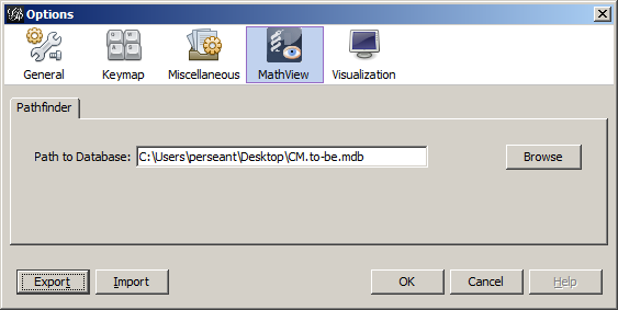
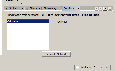
Once this path has been set, click the OK button in the lower right corner of the Options window. This setting will persist and be restored each time MATHView starts up. After this button has been pressed and the options window has closed, the directory path will be displayed in the main Gephi window in the Pathfinder panel.
It is possible to rearrange both the size and locations of all the panels you see on the screen. The default configuration has the large Graph panel in the center and the panels that require less space on both sides. Since neither the Pathfinder panel nor its associated Status Messages panel require much space, they should be located off to one side. To move a panel, use the left mouse button and drag the panel's name tab to the area of the window you want it to be; an outline of the location the window will snap to when released will appear. Once a panel has been moved, that location will be saved and restored the next time the program restarts.
Generating a Pathfinder network from a process model takes just a few steps to generate and configure the display of the network. The configuration of the display attributes only need be done once—the settings will persist when the network is saved and reloaded.
While the Gephi Quick Start Guide and Visualization Tutorial provide more detailed information about many of the valuable features, a few of the most basic items are worth pointing out here.
Gephi provides a targeted zoom
function, using the mouse
wheel. Scrolling the wheel back zooms out, while scrolling the wheel
forward zooms in, both with the perspective vanishing
point centered on the point where the mouse pointer is
located. This, it is possible to zoom out of a graph to see
everything, and then zoom in on an area of interest.
If you want to see the whole graph at once, use the Magnifier
with square corners
icon on the left side of the Graph window.
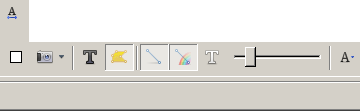
Along the bottom edge of the Graph panel you will see several
controls for setting visual attributes of the graph. Two of these
controls contain the image of a capital T
—the left
toggle controls the visibility of the node labels and the right one
controls the visibility of the edge labels. Click each of these to
set the visibility of the labels as desired.
Initially, the nodes in Gephi are quite small, making them difficult to select. There are two ways to make the nodes large enough to be clicked on.
You can use the following procedure to get larger round nodes:
This method has the disadvantage that any new nodes created (e.g., cluster nodes) will not automatically match the size you've just adjusted everything to. To address that, assuming that node labels have been turned on as above, we can make the nodes automatically resize to match their labels.
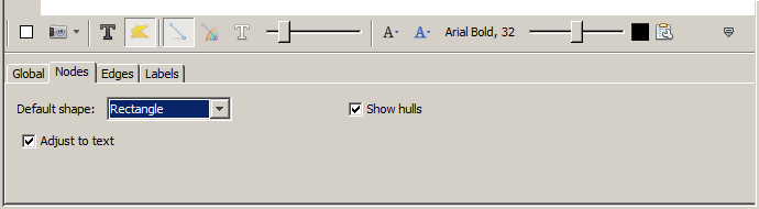
On the bottom right side of the Graph panel there is a small upward
pointing triangle; clicking it opens a panel with more
customizations. Once this panel opens, select the Nodes
tab.
Change the default shape to be Rectangle and check
the Adjust to text check box, so that the labels and node
sizes will stay in sync.
Along the upper left side of the graph window is a vertical strip
of tool icons; three of the more frequently used are the multi-node
selection rectangle (a dotted rectangle), the drag mode tool
(a hand
icon, just below the selection rectangle tool), and
the Nodes attribute
tool, which is the bottom tool icon. All
of these tools are sticky
—that is, they stay in effect
until another is chosen. Drag mode is the default tool chosen on
start-up.
![]()
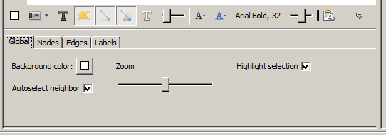
Once in drag mode, left-clicking on a node and dragging it will move it and any attached edges will go with it. Right-clicking and dragging on the background of the window will move the whole graph. If your mouse has a wheel, then zoom in and out are mapped to mouse wheel motion. Two additional options may be useful. If you open the customizations panel (as mentioned above) and look in the Global tab, you will see two check boxes: Highlight Selection and Autoselect Neighbors. If the first is checked, putting the mouse over a node will cause the node and any attached edges to highlight and the rest of the graph to dim. If the Autoselect Neighbors box is also checked, this effect is extended to the nodes at the other end of the edges emanating from the moused-over node.
You can select which edges you want to see in the graph window using the Filters window. Open up Edges from the tree selector, and double-click on Edge Weight, then click on the Filter button. You can now move the left and right slider controls to change the range of edge weights displayed in the graph window. If you click Filter a second time, the filter is turned off.
![]() Caution: The lowest weight edge(s) in the graph will be
displayed with very thin lines, as if their weight were zero,
regardless of their actual weight. In particular, if the edges
visible through the filter have constant weight, all of the
visible edges will be represented as extremely thin lines.
Caution: The lowest weight edge(s) in the graph will be
displayed with very thin lines, as if their weight were zero,
regardless of their actual weight. In particular, if the edges
visible through the filter have constant weight, all of the
visible edges will be represented as extremely thin lines.
Gephi comes with several automatic graph layout algorithms, which can help to visualize the relationships within the graph.
To lay out the graph according to one of these automatic schemes, select the desired layout from the pull-down control in the Layout window. There are several possibilities here; the one we have used the most for our initial work has been Fruchterman-Reingold, which arranges the nodes in a disc with even spacing, with more strongly connected nodes nearer to one another within that fixed pattern.
![]() Caution: The layout algorithm YifanHu's Multilevel
assigns all nodes to unlabeled clusters during its operation, so if
you use that layout, the node labels will disappear.
Caution: The layout algorithm YifanHu's Multilevel
assigns all nodes to unlabeled clusters during its operation, so if
you use that layout, the node labels will disappear.
Once you have selected which layout algorithm you would like to
use, press the green Start
button. While the algorithm is
running, the Start
button will turn into a red Stop
button. Ideally the layout will finish quickly, but sometimes the
layout algorithm never completes. If the graph stops moving before
the algorithm is finished, feel free to press the red Stop
button to accept the algorithm's progress up to that point.
If a filter is in place while the layout algorithm is run, it will only take the visible edges into account. Thus, you may get different layout results depending on what edges are visible.
The multi-node selection rectangle is often used to apply an
operation to a group of nodes all at once. One such operation is to
create a cluster node
or higher-level node that contains the
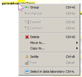
selected nodes as its children. To manually create a cluster, use
the multi-node select tool to sweep a rectangular region that
contains the desired nodes and then right-click on one of the
selected nodes and select Group from the context menu. The
selected nodes will be collapsed into a Group node that has the
default name that looks like Group (N nodes)
,
where N is the number of nodes in the newly created group.
To undo this operation, right-click on the group node and
select Ungroup from the context menu. To expand the group
so that its members are visible, select Expand; to collapse
a group, right-click on one of its members and
select Contract.
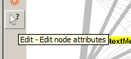
To give the newly created group node a more meaningful name, first select the Edit Node Attributes tool, then select the node whose attributes you want to see or edit. A variety of node attributes will appear in the Edit panel in the upper left part of the top-level window. Type in the new label and hit Enter to set the new label.
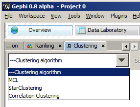
In addition to the standard algorithms supplied by Gephi, MATHView includes the capability to automatically cluster nodes according to the weight of their shared edges. To do this, select Clustering from the Window menu.
Within the clustering panel, first choose the clustering algorithm from the combo box. Available clustering algorithms are Star, Correlated, and MCL.
To the right of the combo box is a Settings button that allows you to configure settings for the chosen algorithm. These settings revert to their default each time an algorithm is selected, so if non-default values are desired it is important to adjust the settings before each run.
At the bottom right of the panel is a Run button—this button is enabled after an algorithm has been selected. Clicking the button invokes the selected algorithm. In case the execution of one of the selected algorithm should take too long (due to incompatible parameters, for example), this same button changes to be a 'Cancel' button during execution.
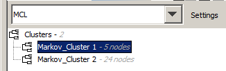
Below the combo box is an area that displays information about clusters recently discovered by the chosen algorithm. The default names given to new clusters are of the form AlgorithmName_SequenceNumber, so new Star Clusters (for example) will be named StarCluster_1, StarCluster_2, etc. To effect these clusters within the graph, right-click on one of the potential clusters' names and from the context menu, select Group. Similarly a cluster can be ungrouped using the context menu.
![]() Caution: The clusters found by the Star Clustering algorithm
might share nodes. Gephi will not allow a node to belong to more than
one group at a time, so you need to be careful, when selecting
clusters for grouping, not to form groups that share
nodes.
Caution: The clusters found by the Star Clustering algorithm
might share nodes. Gephi will not allow a node to belong to more than
one group at a time, so you need to be careful, when selecting
clusters for grouping, not to form groups that share
nodes.
The Star clustering algorithm looks for 'hub' or center nodes that have a higher degree than the average degree of the 'spoke' nodes that the hubs are adjacent to. The 'Star threshold' setting in the settings panel defaults to 0.5. The 'star measure' of a set of nodes (center node + its set of adjacent spoke nodes) is calculated as totalDegree / (centerDegree * centerDegree), where totalDegree is the sum of the degrees of the set of spoke nodes for each hub node (which has a degree of centerDegree). A 'star cluster' is formed when the star measure is less than or equal to the star threshold.
The Correlated clustering algorithm has two numeric parameters—a low limit and a high limit. These are used to filter out edges whose weight falls outside this range. Once these edges have been filtered out, the algorithm partitions the network into a set of connected components, each of which becomes a new cluster. The primary motivation for this algorithm was the observation that pairs, or larger sets, of nodes connected by edges with weight of 1.0 have perfectly correlated usage patterns across business process steps and often make good clusters.
The Markov clustering algorithm description is a bit more complicated. Markov Clustering implements the Markov clustering (MCL) algorithm for graphs, using a HashMap-based sparse representation of a Markov matrix, i.e., an adjacency matrix M that is normalized to one. Elements in a column / node can be interpreted as decision probabilities of a random walker being at that node. Note: whereas we explain the algorithms with columns, the actual implementation works with rows because the used sparse matrix has row-major format.
The basic idea underlying the MCL algorithm is that dense regions in sparse graphs correspond with regions in which the number of k-length paths is relatively large, for small k in N, which corresponds to multiplying probabilities in the matrix appropriately. Random walks of length k have higher probability (product) for paths with beginning and ending in the same dense region than for other paths.
The algorithm starts by creating a Markov matrix from the graph, for which first the adjacency matrix is added diagonal elements to include self-loops for all nodes, i.e., probabilities that the random walker stays at a particular node. After this initialization, the algorithm works by alternating two operations, expansion and inflation, iteratively recomputing the set of transition probabilities. The expansion step corresponds to matrix multiplication (on stochastic matrices), the inflation step corresponds with a parametrized inflation operator Gamma_r, which acts column-wise on (column) stochastic matrices (here, we use row-wise operation, which is analogous).
The inflation operator transforms a stochastic matrix into another one by raising each element to a positive power p and re-normalizing columns to keep the matrix stochastic. The effect is that larger probabilities in each column are emphasized and smaller ones deemphasized. On the other side, the matrix multiplication in the expansion step creates new non-zero elements, i.e., edges. The algorithm converges very fast, and the result is an idempotent Markov matrix, M = M M, which represents a hard clustering of the graph into components.
Expansion and inflation have two opposing effects: While expansion flattens the stochastic distributions in the columns and thus causes paths of a random walker to become more evenly spread, inflation contracts them to favored paths.
This description is based on the introduction of Stijn van Dongen's thesis, Graph Clustering by Flow Simulation (2000); for a mathematical treatment of the algorithm and the associated MCL process, see http://micans.org/mcl//index.html?sec_thesisetc.
Clusters, whether manually or automatically generated, can be exported as Java header files using the Export Clusters option from the File menu. You will be presented with a dialog box to select the directory within which the header files are to be created.
![]() Caution: A common error is to try to enter a file
name, and indeed the dialog box appears to be asking for a file name.
Since more than one file will be created, however, you must select
an existing folder. The dialog box provides folder creation
functionality, if the folder you intend to generate the headers into
does not exist yet.
Caution: A common error is to try to enter a file
name, and indeed the dialog box appears to be asking for a file name.
Since more than one file will be created, however, you must select
an existing folder. The dialog box provides folder creation
functionality, if the folder you intend to generate the headers into
does not exist yet.
One file will be created per cluster, with a file name corresponding to the cluster name. So, if the cluster was named MarkovCluster_1, the file will be named MarkovCluster_1.java.
It is important to note that the cluster names are used directly as the class names, and as such, they should represent valid class names. Thus, they should begin with a capital letter, and contain only letters, numbers, and underscore (_); in particular, no spaces or punctuation are allowed.